Empirical photometric correction applied
In order to check for any remaining systematic effects in the final photometry,
we querried the Archive, collected all normal star observations, and reduced
them in the same way as the young stellar objects.
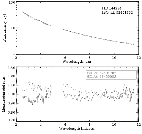
Figure 1 shows a typical result, where the
measured spectrum is compared with the expected one. The latter spectrum was
taken from the ISO calibration data base which includes a compilation of
predicted spectra provided by M. Cohen or P. Hammersley (ISO website). For those
objects not included in the data base we took one of the available models of
a star of identical spectral type, and scaled the values to the K-magnitude of
our object. In our sample of 43 normal star observations no excess due to hot
circumstellar dust is expected (the sample also include the calibrator stars).

Fig.1: Upper panel: Spectrum of the standard star HD 144284 (histogram)
compared with model prediction (solid line). Lower panel: Ratio of
measured flux values to model prediction for two independent observations of
HD 144284.
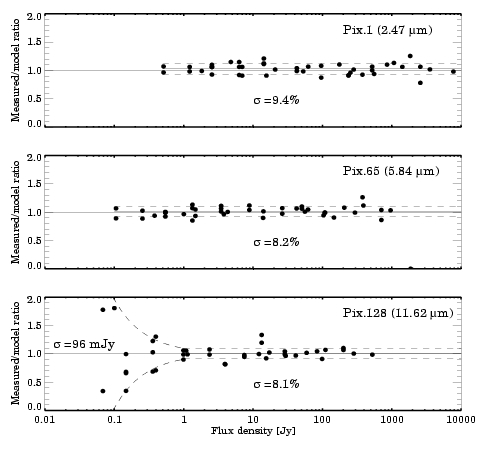
Figure 2 shows the measured-to-predicted ratios of 3 representative pixels
for the whole sample. For each pixel the ratios above a brightness threshold
(usually 5 Jy) were averaged and their standard deviation was computed. For the
faint stars (below 1 Jy) the ratio values became too noise, and we computed
the average and the standard deviation of the [Measured--Predicted] flux
differences. The averages derived this way represent the typical systematic
errors. We decided to correct for these systematic errors by dividing by the
average flux ratio or by subtracting the average flux difference from all
observations. This empirical photometric correction was the last step
of the our post-processing sequence.

Fig.1: Ratio of measured flux values to model prediction for 3 wavelengths
(all normal star observations are included). Uncertainty values representative
of the whole ensemble are computed separately at high flux level (expressed
in %) and at low flux level (in mJy).
