F.3 Variable Flat-Field

After the LTT has been corrected, we then take into account the pixel-to-pixel temporal variations of the detector response. These response variations (that represent $\sim$1-3% of the average flat-field) are observed at various time scales. To go further in the data processing, we try to correct these pixel-to-pixel response variations with a time dependent flat-field $F(x,y,t)$. Flat-field and sky structures are mixed together in $I_{obs}(x,y,t)$ (see Equation F.1) but the flat-field variations can be extracted from the data by estimating $I_{sky}(x,y,t)$ and by taking advantage of the spatial redundancy.

Here are the guidelines of this method:

1. Construct a sky image.
2. Smooth (median smoothing) the sky image with a $10\times10$ window.
3. Compute an ideal cube $I_{sky}(x,y,t)$ by projecting the smoothed sky image on each readout of the data cube.
4. Smooth (median smoothing) $I_{obs}(x,y,t)/I_{sky}(x,y,t)$ on the time axis. The size of the smoothing window should be of the order of the time spent on 5 different sky positions. The result of this smoothing is the variable flat-field.

The sky image of the first GRB observation, obtained with the variable flat-field, is shown in Figure F.3c. The variable flat-field removes almost all periodic patterns due to high-frequency variations of the detector response.

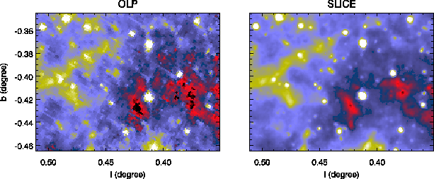
Figure F.4: A small piece of an LW2 image of the ISOGAL survey. Left: image obtained from the standard pipeline data processing (OLP v9.1). Right: image obtained with SLICE, where the spatial redundancy is used to optimise the processing.