|
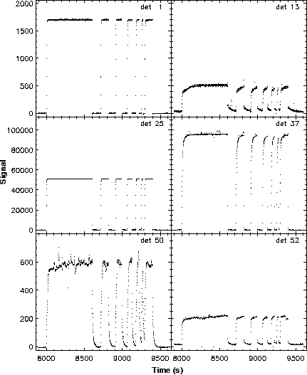
The band 2 (Si:Ga), 4 (Ge:Be), 5 (Si:Ga) and 6 (Ge:Be) detectors used in SWS `remember' their previous illumination history. Going from low illumination to high illumination, or vice versa, results in the detectors asymptotically reaching their new output value. These are referred to as memory effects or transients. Bands 1 (InSb) and 3 (Si:As BIBIB) are not affected by memory effects due to the different detector material used.
Figure 9.1 gives an example from all bands during illumination changes. In this figure it can be seen that bands 2, 4, 5 and 6 have severe memory effects, while bands 1 and 3 show no such effects - these detectors instantaneously reach the signal level corresponding to the new illumination levels.

|
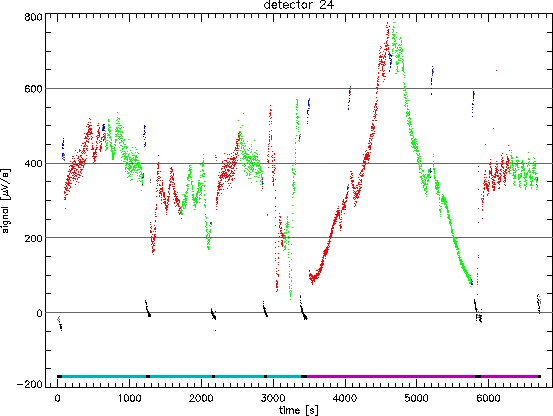
Another example of memory effects is the effect seen in up-down scans of fairly bright sources. For sources with fluxes greater than about 100 Jy memory effects cause the up and down scans in the SPD to differ in response by up to 20% in bands 2 and 4. This effect can be seen in Figure 9.2 for band 2 and in the Figures 9.5 and 9.6 for band 4. Figure 9.2 shows the output of detector 24 against time. Several up-down scans were taken during this measurement, interspersed with dark currents and sometimes reference scans. During a reference scan the grating is moved to a fixed wavelength position to (re)measure the same flux level. This was done to obtain more information on the memory effects, although the scans were never explicitly used for this purpose. The up-down scans have a clear asymmetric shape, the dark currents are not constant and the reference scan do not yield the same flux levels. All this is indicative of serious memory effects.
|
Currently the only memory effects corrected for in the pipeline are those that affect band 2 detectors. They are modelled as changing dark currents. This is mainly discussed in Section 9.2.1. Section 5.3 discusses the general methods used in the dark current subtraction and Section 7.3.3.2 discusses its implementation.
Figure 9.3 shows the result of this in an AAR
after
application of the transients models described in Section
9.2.1. The up and the down scans overlap quite well
and the reference scans find their proper place in the spectrum at 4.5
![]() m and 7.7
m and 7.7 ![]() m.
m.

|
For transient effects in the longer wavelengths detectors (band 4 and both FP bands) see Section 9.2.2.
An adapted version of the Fouks-Schubert model (Fouks and Schubert 1995, [10]) was developed by Do Kester and successfully implemented in the SWS pipeline to correct band 2 data for transient effects. The method brings the errors (of sometimes up to 20%) down to the few percent level.
The Fouks-Schubert model is written for semi-stationary fluxes, where the semi-part reflects the fact that the detectors do not have to be in an equilibrium state when the next flux step takes place. For a spectrometer like SWS the flux changes continuously, with every reset interval, or even every step of the grating scanner, giving a new constant flux level. The detectors are (almost) never in an equilibrium state but that is taken into account in the formula. The original Fouks-Schubert formula was therefore rewritten into a form more suitable for SWS.
Here ![]() is the signal through the detector at time
is the signal through the detector at time ![]() ,
,
![]() is the relaxed signal at time
is the relaxed signal at time
![]() . It is
proportional to the incoming flux.
. It is
proportional to the incoming flux. ![]() is a constant,
to be estimated from the data, and
is a constant,
to be estimated from the data, and
![]() comprises the memory
effects.
comprises the memory
effects.
![]() is dependent on its previous value,
is dependent on its previous value,
![]() , on the present relaxed signal,
, on the present relaxed signal,
![]() , and on
the constants
, and on
the constants ![]() and
and ![]() .
. ![]() is the duration of the
time step from
is the duration of the
time step from ![]() to
to ![]() . The signal is related to the relaxed
signal (or flux) via a constant gain
. The signal is related to the relaxed
signal (or flux) via a constant gain ![]() and a changing dark
current
and a changing dark
current ![]() . It is a fortuitous coincidence that we used this gain
and dark model already in the pipeline. We can identify the product of
. It is a fortuitous coincidence that we used this gain
and dark model already in the pipeline. We can identify the product of
![]() with the incoming flux as it better reflects our
present dark current model of signal = flux + dark. The absorption of
the constant factor,
with the incoming flux as it better reflects our
present dark current model of signal = flux + dark. The absorption of
the constant factor, ![]() , in the subsequent calculations is trivial.
, in the subsequent calculations is trivial.
When the incoming flux is zero, i.e. when measuring with a closed shutter (a
`dark current measurement'), the above expression for ![]() breaks down
yielding 0/0. Using l'Hôpital's rule we find a new expression for
breaks down
yielding 0/0. Using l'Hôpital's rule we find a new expression for ![]() when
when
![]() :
:
This expression decays to zero in a more or less hyperbolic manner as
observed in the Si:Ga detectors. The constant ![]() is the fraction
of the relaxed signal which expresses itself immediately, so
is the fraction
of the relaxed signal which expresses itself immediately, so ![]() is
between 0 and 1. The incoming flux is always positive or zero in case of
a dark current. It follows from Equation 9.2 that the
values of
is
between 0 and 1. The incoming flux is always positive or zero in case of
a dark current. It follows from Equation 9.2 that the
values of ![]() are always positive and so is the signal S. We
measure, however, (dark) values which are negative for some detectors.
So we must conclude that the model is not yet complete, as the zero
level in the data cannot be mapped directly on the zero of the model.
This is not so disturbing as the zero in the data can be changed
somewhat arbitrarily by changing, for instance, the value of `midbit'.
Also the zero level shifts when the gain setting changes or when the
length of the reset interval changes. All these stepwise zero shifts are
artificial in the above sense.
are always positive and so is the signal S. We
measure, however, (dark) values which are negative for some detectors.
So we must conclude that the model is not yet complete, as the zero
level in the data cannot be mapped directly on the zero of the model.
This is not so disturbing as the zero in the data can be changed
somewhat arbitrarily by changing, for instance, the value of `midbit'.
Also the zero level shifts when the gain setting changes or when the
length of the reset interval changes. All these stepwise zero shifts are
artificial in the above sense.
Thus, we expand the model by adding a model zero level
Determining the zero-level function (ZLF) was difficult, as the behaviour at low fluxes is extremely sensitive to the zero level. Piecewise linear functions between dark currents of the same gain setting were used. In this way, the Fouks-Schubert model at low fluxes behaves similarly to the standard dark current subtraction used in all previous pipeline versions, which was deemed correct at low fluxes.
Now we have a (forward) function which relates the measured signal to
the incoming flux in a complicated, non-linear fashion. We only have to
invert the relationship, and as the constant ![]() is quite large
(
is quite large
(![]() 0.8) we can do the inversion iteratively
0.8) we can do the inversion iteratively
where
![]() is calculated with the values of
is calculated with the values of
![]() from
the previous iteration. For most observations the flux stabilises after
half a dozen iterations.
from
the previous iteration. For most observations the flux stabilises after
half a dozen iterations.
In total we have ![]() parameters:
parameters: ![]() ,
, ![]() ,
,
![]() plus the parameters needed in the ZLF.
plus the parameters needed in the ZLF.
![]() is
the value of
is
the value of ![]() before the observation started. The first two
parameters are material constants, i.e. they might be fixed over the
mission and if that is the case they would have to be estimated only
once. The others are related to the flux history in some sense. As this
history is unknown these parameters have to be estimated for each
observation separately. Note however that the ZLF is chosen to be
linear. Consequently for each choice of
before the observation started. The first two
parameters are material constants, i.e. they might be fixed over the
mission and if that is the case they would have to be estimated only
once. The others are related to the flux history in some sense. As this
history is unknown these parameters have to be estimated for each
observation separately. Note however that the ZLF is chosen to be
linear. Consequently for each choice of ![]() ,
, ![]() and
and
![]() the ZLF-parameters can be estimated directly, simplifying the
non-linear search for the other parameters. All parameters, however,
have to be estimated at least once.
the ZLF-parameters can be estimated directly, simplifying the
non-linear search for the other parameters. All parameters, however,
have to be estimated at least once.
To estimate the parameters we use the redundancy in each observation: up-down and 12 detectors covering more or less the same spectral area. The procedure is described in Kester 2001, [22], or García-Lario et al. 2001, [11].
The parameters can be estimated properly when an SPD is used with
sufficient dynamic range between 100 and 5000 ![]() V/s. For fluxes much
larger than 5000
V/s. For fluxes much
larger than 5000 ![]() V/s, other memory effects than the ones we are
modelling become important. On the other hand when the flux range is too
small (
V/s, other memory effects than the ones we are
modelling become important. On the other hand when the flux range is too
small (![]() V/s) not enough memory effects are present to allow
proper extraction of parameters. In that case it is possible, by
keeping the parameters
V/s) not enough memory effects are present to allow
proper extraction of parameters. In that case it is possible, by
keeping the parameters ![]() and
and ![]() fixed and fitting the
others, to get proper transients, which will not be much different from
the dark current the pipeline would yield.
fixed and fitting the
others, to get proper transients, which will not be much different from
the dark current the pipeline would yield.
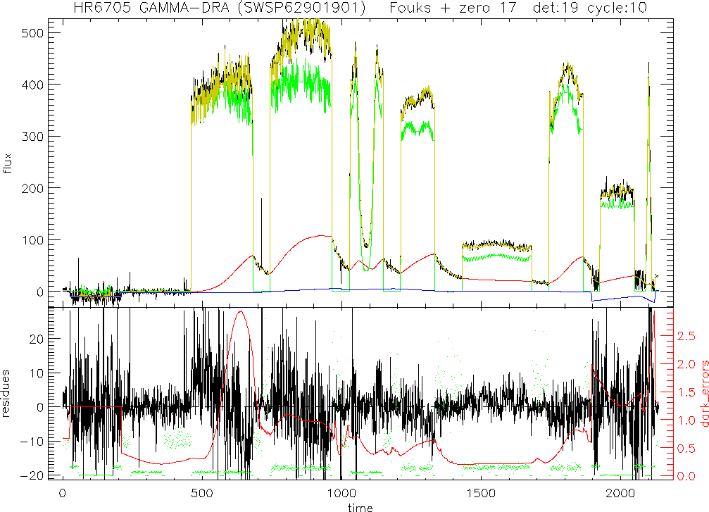 |
Figure 9.4 shows an example how the memory model
changes over time for one detector during an observation of the
calibration star ![]() Dra. In the upper panel the measured data is
plotted in black, the relaxed signal in green (symmetric in up-down),
the transients,
Dra. In the upper panel the measured data is
plotted in black, the relaxed signal in green (symmetric in up-down),
the transients, ![]() , in red and the zero level in blue. Note
that the measured data go below zero and that consequently the model
zero level is also below zero. In yellow the model data (relaxed signal
+ dark) is plotted. They are compared to the true data to calculate
, in red and the zero level in blue. Note
that the measured data go below zero and that consequently the model
zero level is also below zero. In yellow the model data (relaxed signal
+ dark) is plotted. They are compared to the true data to calculate
![]() . The memory model has some real impact whenever the flux is
more than a few 100
. The memory model has some real impact whenever the flux is
more than a few 100 ![]() V/s, e.g. between time 500 and 1000. On the
other hand when the flux is below 100
V/s, e.g. between time 500 and 1000. On the
other hand when the flux is below 100 ![]() V/s, e.g. around time 1500, a
straight line between the surrounding dark currents is equally good. In
the lower panel the residues are plotted in black, the weights of the
points in green (scale on the right). There are some systematic
effects, but most of the high noise at high flux has to do with the
fact that the measured spectrum is fluctuating (or fringing) severely
which cannot be properly followed during the rebinning. In red in the
lower panel (to be read on the red scale) is a Monte-Carlo estimate of
the error in the memory model.
V/s, e.g. around time 1500, a
straight line between the surrounding dark currents is equally good. In
the lower panel the residues are plotted in black, the weights of the
points in green (scale on the right). There are some systematic
effects, but most of the high noise at high flux has to do with the
fact that the measured spectrum is fluctuating (or fringing) severely
which cannot be properly followed during the rebinning. In red in the
lower panel (to be read on the red scale) is a Monte-Carlo estimate of
the error in the memory model.
We determined the parameters ![]() and
and ![]() from 65 observations
of
from 65 observations
of ![]() -Dra and checked it afterward on all SWS01 observations which
had a median flux in band 2 higher than 100
-Dra and checked it afterward on all SWS01 observations which
had a median flux in band 2 higher than 100 ![]() V/s. We searched for
time variations in the parameters, for variations as function of the
flux level and even for variations with temperature, using an extension
of the FS formalism. None of the variations was very significant. So we
settled for one set of parameters for all of the band 2 detectors,
presented in Table 9.1. More details in Kester 2001,
[22], or García-Lario et al. 2001,
[11].
V/s. We searched for
time variations in the parameters, for variations as function of the
flux level and even for variations with temperature, using an extension
of the FS formalism. None of the variations was very significant. So we
settled for one set of parameters for all of the band 2 detectors,
presented in Table 9.1. More details in Kester 2001,
[22], or García-Lario et al. 2001,
[11].
All pipeline calculations are done with these two parameters fixed. The
parameters of the zero-level function and the value for ![]() are
estimated for each observation separately.
are
estimated for each observation separately.
When we have arrived at the minimum value for ![]() the standard
deviations and covariance matrix for all parameters is calculated,
using a Gaussian approximation at
the standard
deviations and covariance matrix for all parameters is calculated,
using a Gaussian approximation at
![]() . Typical errors that
we find in a good observation are a few per thousand in
. Typical errors that
we find in a good observation are a few per thousand in ![]() , a few
percent in
, a few
percent in ![]() and of the order of 1
and of the order of 1 ![]() V/s in the other
parameters (
V/s in the other
parameters (![]() and the ZLF). However, we are not so much
interested in the formal errors in the parameters but much more in the
effects they have on the calculated dark current. We use a Monte Carlo
scheme where the dark current is calculated 25 times, each time with
another randomized set of parameters, drawn from a multidimensional
Gaussian distribution representing the full covariance matrix. At each
sample the standard deviation of these 25 dark currents is taken as the
formal error. See the red line in the lower panel of Figure
9.4.
and the ZLF). However, we are not so much
interested in the formal errors in the parameters but much more in the
effects they have on the calculated dark current. We use a Monte Carlo
scheme where the dark current is calculated 25 times, each time with
another randomized set of parameters, drawn from a multidimensional
Gaussian distribution representing the full covariance matrix. At each
sample the standard deviation of these 25 dark currents is taken as the
formal error. See the red line in the lower panel of Figure
9.4.
The transient effects in band 4 and in both FP bands can be about as severe as in band 2. Various effects can be seen in Figure 9.5. It is an SWS01 speed 4 observation of K3-50. At the start of the up-down scan (at the longer wavelength side) we see a transient. Some detectors, like 37, display a so-called `hook' effect, some rise faster than others, seeming to get earlier to their relaxed state than the others. At the shorter wavelength there also seems to be some hysteresis effect, where the second part (the down scan in red) seems to stall before getting into the rising mood.
Figure 9.6 displays the same object but then in an SWS01 speed 2 observation, i.e. scanning the spectrum 4 times as fast. It shows the same general trends as in Figure 9.5. In the time domain all detectors react in exactly the same way, which means that in the spectral domain it seems much slower. Both the hook and rise at the start and the hysteresis just after the turning point can be seen. This speed 2 observation has much more glitches; it might have been taken in a more unfavourable part of the orbit. Note that these glitches have their tail, if any, in the time direction, to the left for the up scans (black) and to the right for the down scans (red).

|
Unfortunately we do not have a proper model to correct for transients in band 4. The FS model applies only to Si:Ga detectors as only for these detectors the assumptions are valid which simplified the full set of interdependent differential equations that describe transients in general. With these assumptions these equations can be integrated into the closed system which yield the FS model. In the future it might be possible to extend the FS equations with first order corrections, which then might successfully be applied to band 4 detectors too.
For the FP detectors (Si:Sb and Ge:Be) the transients can be as serious as in band 4 (Ge:Be). However due to the fact that the flux levels seen by these detectors are generally quite low, the problem is not as severe as in band 4. This is a fortunate situation as we will never be able to correct for transients because we do not have up-down scans for the FPs. The FP scanners could only be driven in one direction with full paralellisation of the meshes. So transient information and spectral information is inextricably mixed.
The combined effects of reference scans (described in Section 3.2.2) and detector memory effects produced from band 2 and band 4 detectors during SWS06 observations can be seen in Figure 9.2. Reference scans were introduced to get a handle on the memory effects but as such they were never used due to the lack of an algorithm to do so. Quite early in the mission the number of reference scans per SWS06 was reduced so that only long SWS06 observations had any of them during the up-down scans. They are still present at the beginning and end of an up-down scan. The number was reduced because of the upsetting effect the reference scans had on the rest of the scan.
In band 2 most of the harmful effect of reference scans is removed by the application of the FS model as can be seen in Figure 9.3. In band 4 it just compounds to the transient problems that are already present.
In the document by Leech & Morris 1997, [27], examples of such effects are given and suggestions what to do when they occur9.1.
Glitches are caused by such events as fast moving electrons and ions inside the Earth's magnetic field hitting the detectors. Whatever causes a glitch, the effect of one is a sudden change in the output voltage which causes a step (a `glitch') in the affected ramp. Most glitches cause an increase in the output voltage, but some can cause a decrease. For small glitches (the majority) the slopes before and after the glitch are indistinguishable from each other. Figure 2.7 shows an example of a glitch in the 24Hz ERD data in the middle of the second ramp of a measurement.
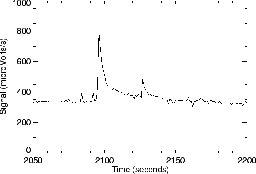
Some glitches, however, are large and have effects that lasts for a long
time (they have tails). These tails are especially seen in band 4, due
to the detector material and operating conditions, and are probably due
to memory effects, see Section
9.2. Figure 9.7 shows two
examples of band 4 glitches in the SPD.
In both cases the detector
requires a long time to stabilise. Note that a strong glitch in one
detector can affect other detectors in the same detector array due to
cross-talk. More examples of glitches (and tails) can be seen in Figures
9.5 and 9.6. In Figure
9.5 a much rarer negative glitch (with tail) is seen
in detector 37 near 42 ![]() m.
m.
Both FP bands are even more affected by glitches than band 4. Their detectors are somewhat larger in size and thus catch more cosmic rays. See Figure 9.1.
Derive-SPD attempts to correct for glitches, and for details of how this is accomplished see Section 7.2.8. No attempt is made to correct for tails.
|