3.7) The PIA Mapping Simulation System
We have developed a mapping simulation system within PIA, capable of generating
sky images with several point / extended sources on a flat / gradient
background and simulating what ISOPHOT would have recorded under certain
instrument and spacecraft raster configurations. While the benefits
of performing simulations for accessing the efficiency, accuracy, confusion
level, etc., on different mapping algorithms and deconvolution techniques
in and outside PIA are mostly of interest to calibrators and instrument
specialists, it is also very important for a general observer because this
highly user friendly system provides the possibility of simulating his/her
observation by matching the selected observing mode.
The system can be used for testing the following:
validity of theoretical/experimental beam profiles
detection limits and confusion levels
transients and glitches simulated into SRD level data
different algorithms in relation to different observation configurations
(improving data analysis)
reliability of obtained results by real observations
The system is divided into three main stages:
sky simulation : a portion of the sky as well as the user defined
number of sources with their respective positions in the sky, fluxes /
brightness and sizes (circular and bar structures are included ) are defined.
The choice between a flat or a gradient background is also available.
Convolution with the footprint of a selected filter yields an image of
the convolved sky in addition to the pure sky. These images together
with the parameter set used to create them are the products of this portion
of the simulation, which can be saved as data entities for reuse at any
time.
observing mode specification : the observing mode is defined together
with the raster parameters (number of raster legs and points per leg, distance
between legs and points, central position of the raster). Both the
orientation of raster vs sky as well as the orientation of spacecraft vs
sky are necessary for establishing the exact positioning of the detectors
(and hence the "measured" flux) on the sky at any step of the observation.
The result is an AAP level data structure which can be used within the
PIA environment as any real observation, e.g. deriving the corresponding
image.
instrumental effects : the expansion of every spatially "measured"
point into a time series of signals as would have been recorded by a real
observation is done together with the inclusion of instrumental effects,
like the transient behavior of the ISOPHOT detectors, the disturbances
produced by cosmic rays, different detector pixel response and a random
noise contribution. The product, a SRD data structure, can also be
ingested into PIA for virtually simulating the data analysis.
The parameters included in all three stages of the simulation system are
kept in configurable tables, so that changes can be easily made from dedicated
GUIs. The model for the transient behavior (by default the so called
"offset exponential function" as explained in the section
3.3.6) can be replaced by any other model function.
The PIA mapping simulation system includes a widget based graphical
user interface, with dedicated menus for each of the three parts of the
system, as mentioned above. Visualization of the created sky images
with superimposed raster and detector pixel positions is also accessible
from the main menu. The visualization tools attached to this GUI
are common to the PIA mapping system, thus offering the user the main IDL
capabilities with respect to image display and manipulation from comprehensive
menus.
3.7.1) The PIA Map Simulation Window
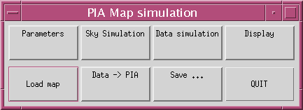
This section describes in detail the PIA Map Simulation window shown in
Figure
1 and its pull-down items. It appears when you click on the
"Simulator" button on the PIA Top Window. This window shown below
will be referred to as the "main window" in the following sections of 3.7.

FIGURE 1: The PIA Map Simulation Window
Parameters
This pull-down item offers the following options:
Edit/change sky map parameters
This brings up the PIA Map Simulation Parameters window shown in Figure
2.
Edit/change data parameters
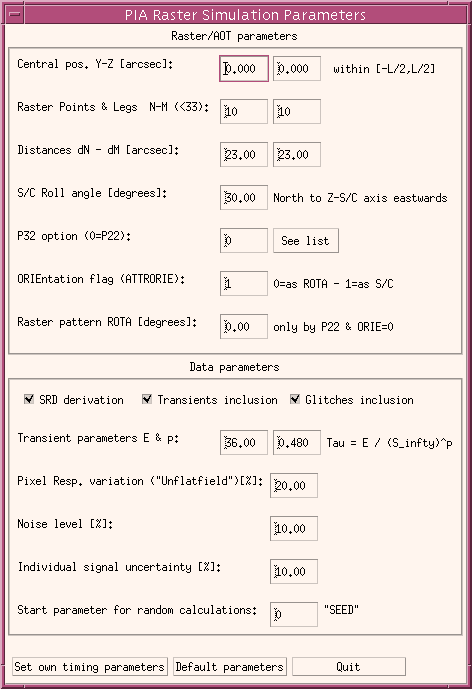
This brings up the PIA Raster Simulation Parameters window shown in
Figure
6.
Sky Simulation
This pull-down item offers the following options:
Using parameter table
This will run the sky simulation using the parameters specified with
the
PIA Map Simulation Parameters window.
Using graphic derivation
This starts the graphic derivation of the sky simulation using the IDL
prompt. With this option, the user is asked to specify the necessary
parameters at the IDL prompt by answering series of questions. As
the inputs are made, the program shows displays and information to guide
the user along. Hence, you are encouraged to try this graphic version
to familiarize yourself with the sky simulation system.
Data Simulation
This pull-down item offers the following options:
Using parameter table
This will run the data simulation using the parameters specified with
the
PIA Raster Simulation Parameters window.
Using graphic derivation
This starts the graphic derivation of the data simulation whose end
products are AAP and SRD data structures. With this option, the user
is asked to specify the necessary parameters at the IDL prompt by answering
series of questions. As the inputs are made, the program shows displays
and information to guide the user along. Hence, you are encouraged
to try this graphic version to familiarize yourself with the raster (AAP
data) simulation system.
Display
This pull-down item offers the following options:
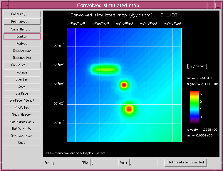
Convolved Sky Image (Jy/beam)
This shows the simulated sky convolved with the footprint of the selected
filter in units of Jy/beam. For example, see the Figure
4.
Convolved Sky Image (MJy/sr)
This shows the simulated sky convolved with the footprint of the selected
filter in units of MJy/sr. This is exactly the same as the previous
image except for the units (MJy/sr instead of Jy/beam).
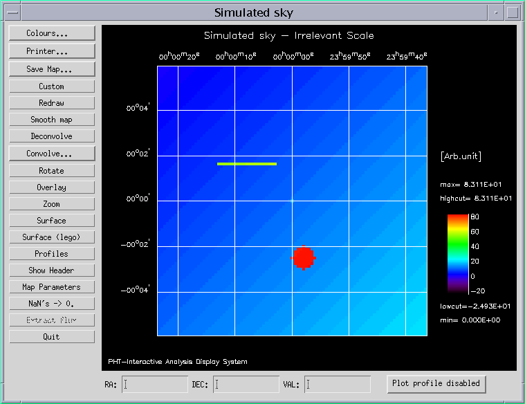
Pure Sky Image
This shows the simulated sky (ideal image) in arbitrary units, see Figure
3. Please note that the scale is meaningless in this image.
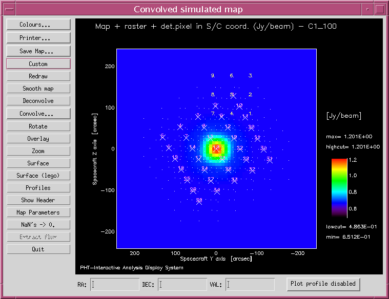
Image + Measured Positions
This shows the simulated sky convolved with the footprint of the selected
filter in units of Jy/beam plus the user defined raster positions.
For example, see the Figure 8.
... + Det.Pixel pos. (in S/C coord) (Jy/beam)
This shows the simulated sky convolved with the footprint of the selected
filter in units of Jy/beam plus the user defined raster positions in the
spacecraft coordinates instead of sky coordinates. For example, it
looks like Figure 9 (except that
the unit is in Jy/beam).
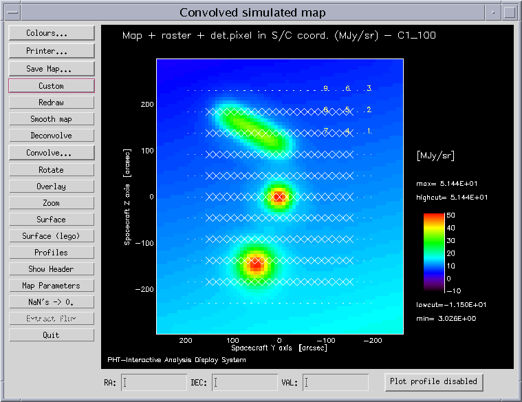
... + Det.Pixel pos. (in S/C coord) (MJy/sr)
This shows the simulated sky convolved with the footprint of the selected
filter in units of MJy/sr plus the user defined raster positions in the
spacecraft coordinates instead of sky coordinates. For example, see
the Figure 9.
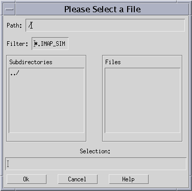
Load map
This calls the Please Select a File window as shown below.

Please specify the name of the file containing the saved simulated
map and its directory path.
Data -> PIA
This pull-down item offers the following options:
AAP -> PIA
Select this option to load the generated AAP data into the PIA buffer.
SRD -> PIA
Select this option to load the generated SRD data into the PIA buffer.
Save ...
This pull-down item offers the following options:
Generated map
This calls the Please Select a File for Writing window, which asks for
a filename (and directory) under which the generated map will be saved
(a default name is proposed).
Generated AAP
This calls the Please Select a File for Writing window, which asks for
a filename (and directory) under which the generated AAP data will be saved
(a default name is proposed) in internal PIA format.
Generated SRD
This calls the Please Select a File for Writing window, which asks for
a filename (and directory) under which the generated SRD data will be saved
(a default name is proposed) in internal PIA format.
The proposed default name has the following format: "C1" or "C2"
depending on the detector used, followed by "99" to differentiate
it from real observations, and the remaining digits represent the time
the data was simulated (i.e., the each set of two digits is in the order
of the month, date, hour and minute). For example, "C19906171703"
can be decoded as a simulated data (looking at the "99" following
the "C1") using the C100 detector created on June 17 at 17:03 or
5:03 PM.
QUIT
3.7.2) Sky Simulation
To complete a sky simulation, you must first define the necessary parameters
either using the PIA Map Simulation Parameters
window in Figure 2 or using
the IDL prompt for graphic derivation. Then, select the appropriate
option under the "Sky Simulation" button in the
PIA Map Simulation window; choose the first option, "Using parameter
table" if you defined the parameters using the
PIA Map Simulation Parameters window or choose the second option, "Using
graphic derivation" if you would like to run the sky simulation graphically
by making inputs at the IDL prompt. Finally, you can examine the
results (pure sky image and convolved sky images as shown in Figure
3 and Figure 4 respectively) using the
"Display" button.
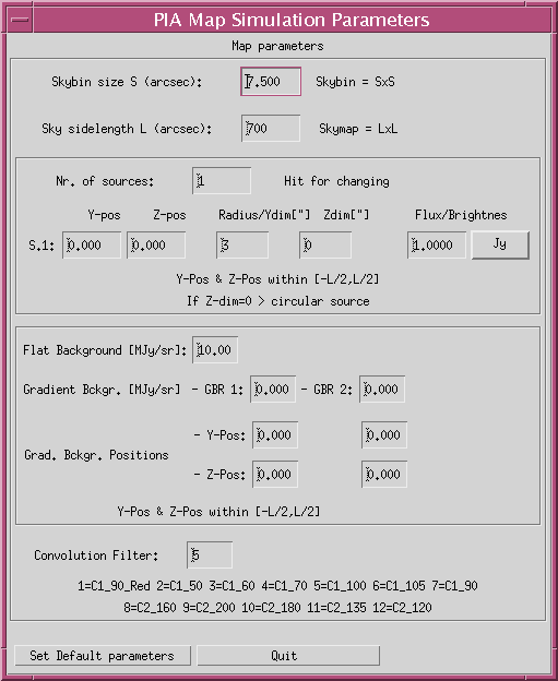
Using the PIA Map Simulation Parameters window
Selecting the "Edit/change sky map parameters" under
the "Parameters" on the main window brings up the PIA Map Simulation
Parameters window shown in Figure 2. See the
detail on each parameter below.

FIGURE 2: The PIA Map Simulation Parameters
window
Skybin size S (arcsec) and Sky sidelength L (arcsec):
For now, the skybin size is fixed as 7.5 arcsec, but you can choose the
size of the sky by specifying the side-length in arcsec. The simulated
sky is always square in shape.
Nr. of sources: Enter the number of sources you would like
to create, and then you must hit the Enter button to modify this window
to accommodate that number of inputs. You can create circular or
bar structures, and you also have the option of entering either the flux
or brightness for each. Specify the position of each source, and
enter their sizes (Z-dim = 0 for circular sources). Don't forget
to select the correct option, Jy or MJy/sr, for each Flux/Brightness value
you enter. For a point source, simply make the size small enough.
Flat Background [MJy/sr]: Enter the brightness for a flat
background. If you don't want a flat background, change the default
value of 10.00 MJy/sr to 0.00 MJy/sr.
Gradient Bckgr. [MJy/sr] and Grad. Bckgr. Positions:
Enter the brightness values at two different locations on the sky, and
the gradient background will be interpolated between these values.
We suggest that you choose the diagonally opposing corners of the sky.
Convolution Filter: Choose the number corresponding to the
filter you would like to use. For example, the number 5 represents
the C100_100 micron filter.
Click the button, "Set Default parameters" to change back to default
parameters or click on the "Quit" button to use the inputs you made
on this window.
Running the sky simulation
If you would like to use the values specified on the parameters table,
then simply click on the option, "Using parameter table" under the
"Sky Simulation" button on the main window. When the sky simulation
is completed, you can view the results (i.e., the pure sky image and the
convolved sky images) using the "Display" button.
If you would like to run the sky simulation graphically at the IDL prompt,
simply click on the second option, "Using graphic derivation" under
the "Sky Simulation" button and answer the proposed questions at
the IDL prompt. The results will be displayed as the necessary inputs
are made, so you can follow the program graphically.
Viewing the sky simulation results
When the sky simulation is completed regardless of the method you used
(using parameter table or using graphic derivation), the results are accessible
from the main window using the "Display" button (only the first
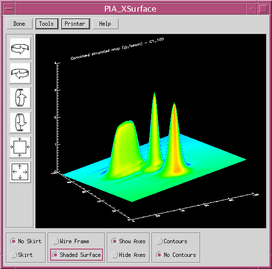
three options are available). The Figure
3 shows an example of a simulated pure sky image, the Figure
4 the convolved sky image in Jy/beam, and the Figure
5 the surface plot of the convolved image. This example case
shows three different sources: a point source at the center of the sky,
a extended circular source and a bar structure. The available visualization
tools are common to the PIA mapping system, thus offering the user the
main IDL capabilities with respect to image display and manipulation from
comprehensive menus.

FIGURE 3: The Pure Sky Image of three different sources

FIGURE 4: The Convolved Sky Image in Jy/beam. The
pure sky image in Figure 3 was convolved with
C100_100 filter as shown in the plot title.

FIGURE 5: The surface plot of the Figure
4. This is produced using the "Surface" button in Figure
4.
Now you can save the generated map by selecting the "Generated map"
under the "Save ..." button on the main window, which calls the
Please Select a File for Writing window. A default name is proposed.
3.7.3) Data Simulation
The observing mode is specified with the raster parameters which include
the number of raster legs and points per leg, distance between legs and
points, central position of the raster, and different rotation angles (all
these will be explained in detail later). The aim is to establish
the exact positions of the detector pixels (and hence the "measured" flux)
on the simulated sky at all specified raster positions. The result
is an AAP level data (and a SRD level data if the user wants it) which
can be used within the PIA environment like any real observation data.
The steps involved in the data simulation are very similar to those
involved in the sky simulation. First, you must define the necessary
parameters either using the PIA Raster
Simulation Parameters window in Figure
6 or using the IDL prompt for graphic derivation. Then, select
the appropriate option under the "Data Simulation" button in the
main window; choose the first option, "Using parameter table" if
you defined the parameters using the PIA
Raster Simulation Parameters window or choose the second option, "Using
graphic derivation" if you would like to run the data simulation graphically
by making inputs at the IDL prompt. Finally, you can examine the
results (the measured positions superimposed on the convolved sky image
in the sky coordinates or the same in the spacecraft coordinates as shown
in Figure 8 and Figure
9 respectively) using the "Display" button. Also, you
can load the generated AAP and SRD data into the PIA buffer or save it
to a file.
Using the PIA Raster Simulation Parameters window
Selecting the "Edit/change data parameters" under the "Parameters"
button on the main window brings up the PIA Raster Simulation Parameters
window shown in Figure 6. See
the detail on each parameter below.

FIGURE 6: The PIA Raster Simulation Parameters window
Raster/AOT parameters
-
Central pos. Y-Z [arcsec]: Enter the central position of the
raster. The first box is for the horizontal coordinate and the second
box for the vertical coordinate in the convolved sky image. The default
has the raster centered at the origin.
-
Raster Points & Legs N-M (<33): Specify the number
of raster points and legs. If you plan to simulate a P32 observation,
you should consider its use of the chopper (i.e., don't make the number
of points too large). Although the limit is 32, real observations
don't use a dimension quite so large.
-
Distances dN - dM [arcsec]: If you choose to do a P22 observation,
specify the distance between the consecutive raster points and legs in
arcsec. This information is irrelevant if you are simulating a P32
observation.
-
S/C Roll angle [degrees]: Enter the angle of rotation for
the spacecraft with respect to the sky in eastward direction from the north.
The detector orientation (i.e., the raster pattern in most cases) will
be rotated through this angle in the counterclockwise direction from the
north in the convolved sky image, except for the special P22 case as discussed
below. The rotation is pivoted at the center of the raster.
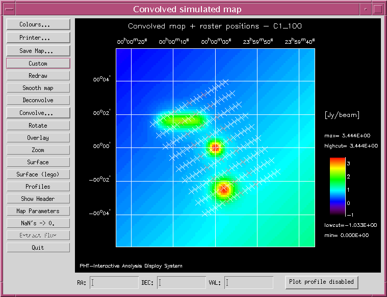
For example, a P32 observation of 3 x 9 raster with a roll angle of 30
degrees is shown in the
Figure 8.
-
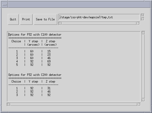
P32 option (0=P22): If you opt to do a P32 observation you
need to choose the raster step size from the choices given in the Figure
7 which is displayed when you click on the "See list" button.
For a P22 observation, use the default value of 0.
-
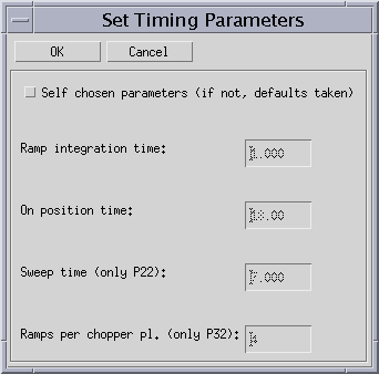
If you are familiar with the timing parameters and would like to modify
them, then click on the button, "Set own timing parameters" to call
the following the Set Timing Parameters window.

-
Click on the "Default parameters" button to revert back to the default
values or click on the "Quit" button to use the inputs and modifications
you have made.
Running the data simulation
If you would like to use the values specified on the parameter table, then
simply click on the option, "Using parameter table" under the "Data
Simulation" button on the main window. When the simulation is
completed, you can view the results (i.e., the convolved sky image plus
the measured positions either in the sky coordinates or in the spacecraft
coordinates) using the "Display" button.
If you would like to run the data simulation graphically at the IDL
prompt, simply click on the second option, "Using graphic derivation"
under the "Data Simulation" button and answer the proposed questions
at the IDL prompt. The results will be displayed as the necessary
inputs are made, so you can follow the program graphically.
Viewing the data simulation results
When the data simulation is completed regardless of the method you used
(using parameter table or using graphic derivation), the results are accessible
from the main window using the "Display" button (the last three
options become available). The Figure
8 shows an example of the "Image + Measured Positions" option
under the "Display" button. This shows the convolved sky image
plus a simulated P32 observation of 3x9 raster rotated through 30 degrees.
The white crosses show all the measured positions (i.e., including the
chopper positions) and the raster points are represented with reddish crosses.

FIGURE 8: An example of "Image + Measured Positions"
display.
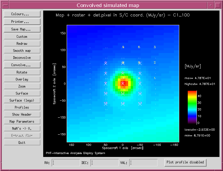
The Figure 9 shows an example
of the "... + Det.Pixel pos. (in S/C coord) (MJy/sr)" option under
the "Display" button. Note that the "... + Det.Pixel pos.
(in S/C coord) (Jy/beam)" is exactly the same as this one except for
the unit, Jy/beam instead of MJy/sr. The Figure
9 is basically the same as the Figure
8 except that it is in the spacecraft coordinates instead of the sky
coordinates (hence, usually zoomed in). Also, it shows the pixel
centers at the first raster position with the numbers 1 - 9.

FIGURE 9: An example of "... + Det.Pixel pos. (in S/C
coord) (MJy/sr)" display
Now, you can save the generated AAP or SRD data to a file by using the
"Generated AAP" or "Generated SRD" under the "Save ..."
button on the main window. This calls the Please Select a File
for Writing window and proposes a default name. You also have the
choice to load it into the PIA buffer using the "AAP -> PIA" or
"SRD -> PIA" under the "Data -> PIA" button, so that you
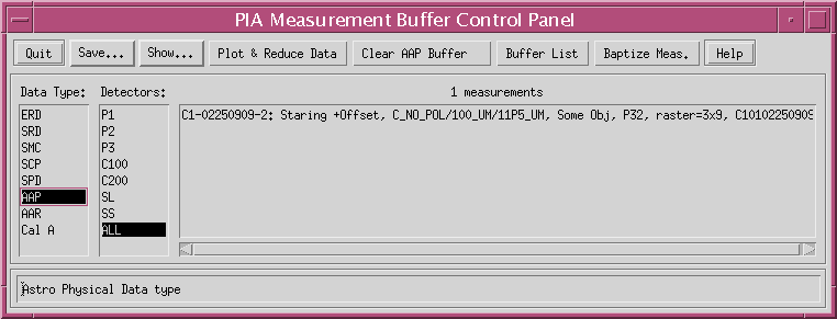
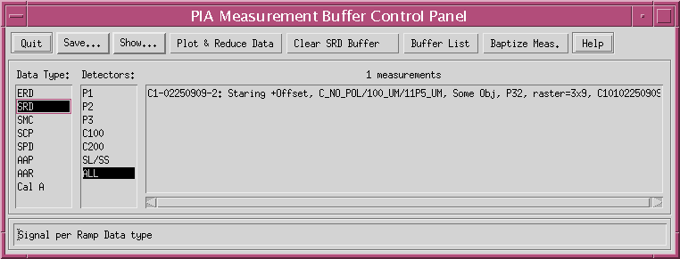
can use it like any other real observation. The Figure
10 shows a simulated AAP data in the PIA buffer, and the Figure 11
shows a simulated SRD data in the PIA buffer.

FIGURE 10: A simulated AAP data loaded into the PIA buffer

FIGURE 11: A simulated SRD data loaded into the PIA buffer
3.7.4) Instrumental Effects
The production of a SRD data involves the expansion of every spatially
"measured" point (AAP data) into a time series of signals as would have
been recorded by a real observation done together with the inclusion of
instrumental effects, like the transient behavior of the ISOPHOT detectors,
the disturbances produced by cosmic rays (glitches), different detector
pixel response ("unflatfielding") and a random noise contribution.
After placed into the PIA buffer, this SRD data can virtually simulate
the data analysis. The following example of a simple P22 observation
shown in the Figure 12 is used to demonstrate
this point visually.

FIGURE 12: A simple P22 observation of 3 x 5 raster
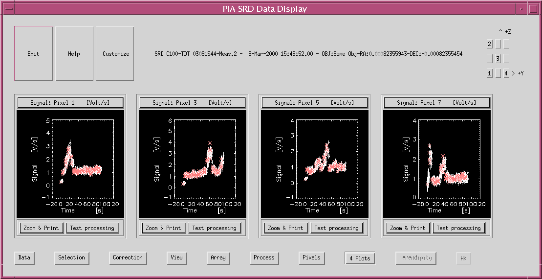
The following Figure 13 shows the generated
SRD data from the simulated P22 observation in the Figure
12. The value of 10.0 % was used for all of the following parameters:
the pixel responsivity variation, noise level, and the individual signal
uncertainty. Also, both transients and glitches were added.
The added glitches should be residual glitches that would not have been
removed from the ERD level correction; hence, the glitches you see in this
simulated SRD data have moderate values.

FIGURE 13: The PIA display of the SRD data derived from
the simulated P22 observation in the Figure
12
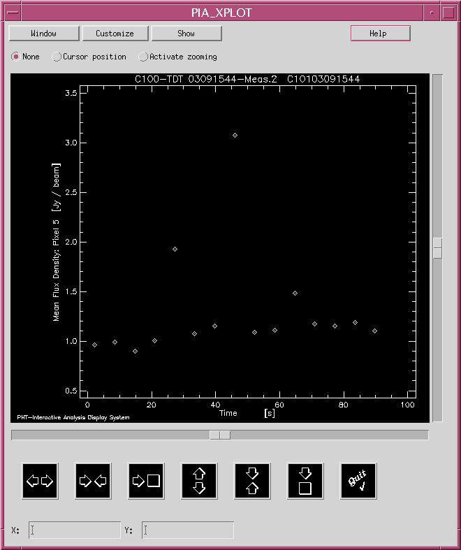
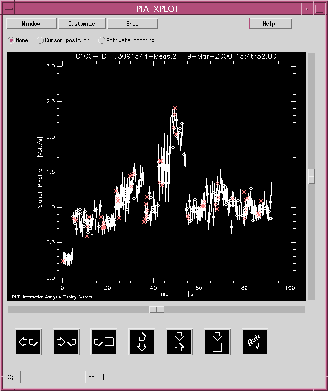
The following Figure 14 and Figure
15 visually demonstrate the addition of instrumental effects to the
AAP data in the Figure 14 to simulate a
SRD data in the Figure 15.

FIGURE 14: The zoomed image of the AAP data of a certain
pixel. This is from the observation shown in Figure
12.

FIGURE 15: The zoomed image of the SRD data of a certain
pixel corresponding to the AAP data shown in the Figure
14. This is from the observation shown in the Figure
12.
Chapter history:
| Date |
Author |
Description |
| 28/02/2000 |
Min Hur (IPAC) / Carlos Gabriel (ESA) |
First Version |
| |
|
|
|
|
|
|
|
|
|
|
|
|
|
|
|
|
|
